In this example we will learn how to optimize delivery lead time, taking into account trade-offs of using faster and more expensive delivery methods against paying penalties for extending delivery time.

We consider a supply chain of the company which buys products from the manufacturer and sells them to the customers on the territory of the US. The considered supply chain contains:

• Supplier – manufacturer of the products in Detroit.
• 11 distribution centers – warehouses where products are stored before being sent to the customers.
• 100 customers distributed across the US.

The customers are placing orders in the morning and are expecting to receive the products by the end of that day. The ordered products are sent to the customers from the DCs. If the order is not delivered by the end of the day, the company pays a penalty (10% of the product's price) to the customer for the late delivery.

The company uses trucks as the primary delivery method, but if the estimated truck delivery time exceeds 2 days, then the cargo plane is used to deliver the ordered products on the next day.

Find the best combination of vehicle types to deliver products from DCs to the Customers considering the lead time constraints, and penalties.

To create the required delivery scheme, we defined 4 vehicle types:

• Truck – regular trucks to deliver product from the Supplier to DCs.
• This day truck – a smaller truck, which is used to deliver products to the customers the same day they were ordered.
• Next day truck – it is used to deliver products that can't be delivered within the same day the customer placed an order. So, the products will be delivered on the next day.
• Next day plane – a cargo plane, which delivers a product that cannot be delivered by the truck within 2 days.

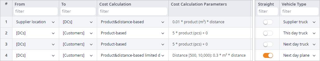
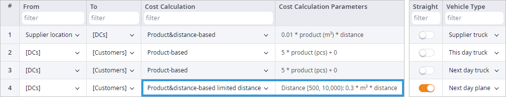
Since the last three vehicle types deliver products to the customers, we create a path from the DCs group to the Customers group for each of them. They differ in Cost calculation Parameters, Transportation Time, and Straight path selections.

The truck delivery costs are the same since the same truck type is used in these two paths. The plane delivery path is more expensive, and it will be set as a straight route, since the plane does not need to follow the roads.

Since the company must pay penalties for not delivering products on the same day they were ordered, we need to add penalty calculation.

To calculate the penalty we can use the revenue that the company received for the products, which were delivered on the next day, and multiply it by the value of the penalty (10% in this case). This can be done in three steps.

In the first step we will make certain preparations for revenue estimation. We have defined flows for every vehicle type in the Product Flows table, set product combinations, assigned meaningful labels for them (to later use them in the Custom Constraints table).

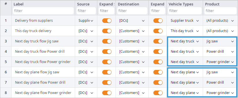
With the second step we will calculate revenues for each product, and then we will sum them up. Now that we have labeled flows, we have the number of products delivered to customers on the next day. To find the revenue we need to multiply the flows by the selling price of the products. We will do it using the Custom Constraints table.

Let us look at the first custom constraint. On the Left-Hand Side, we assigned the name for the expression on the Right-Hand Side. If we open the expression from the Right-Hand Side, we will see that it is a Linear expression with two variables and corresponding coefficients. We can add as many variables as we want, and they all will be summed up considering the coefficient of the variables. In this case, we want to sum two variables, which represent the number of Power grinders delivered by the Next day truck and the Next day Plane. Each of these variables is multiplied by the selling price of one Power grinder ($120) as a coefficient.

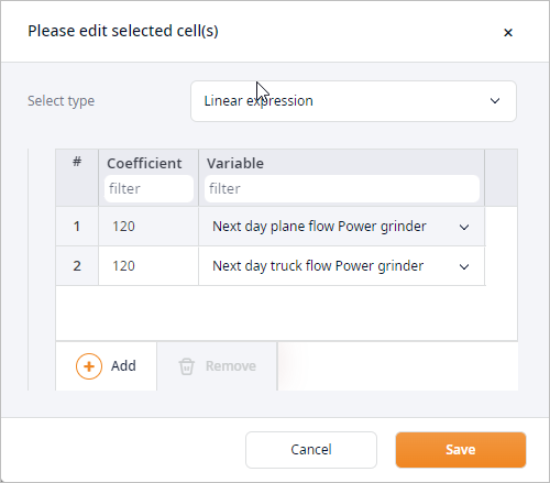
The next two custom constraints are defined in the same way.

The fourth custom constraint helps to sum the revenues calculated by each product into one variable named Next day delivery revenue. That's it for step two.

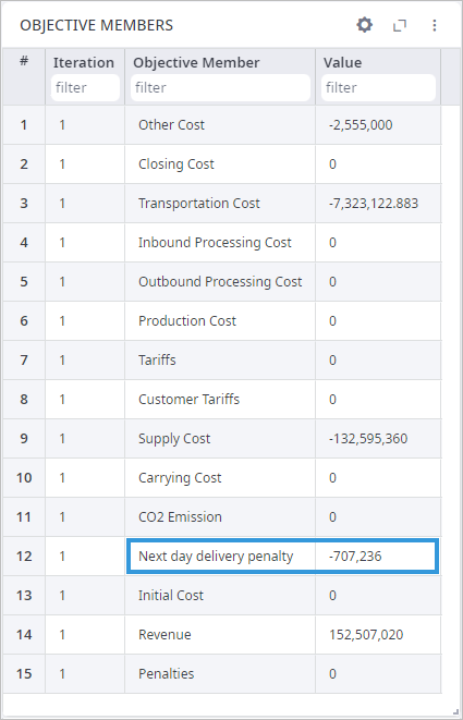
In the third step we will calculate the value of the penalty and add it to the objective of the Network Optimization experiment. Since the penalty affects the financial results, we have to use the Objective Members table.

To consider the penalty in the objective function we need to create a new Objective Member named Next day delivery penalty. In the expression column, we specify that the penalty is calculated as revenue for the next day delivery multiplied by the value of the penalty

Where:

• Next day delivery revenue — the variable
• value of penalty — 10%, which is set as a negative number because the penalty is paid by the company.

In anyLogistix there is no direct way to take time into account in the Network Optimization experiment. The goal of this example is to optimize the supply chain based on the delivery time, so we need to find a way of defining constraints to run the experiment.

We will optimize our supply chain by considering the maximum distance that 1 truck can cover during the day (500 miles), and not the number of days it takes to deliver a product. This way we can set constraints for the delivery process and run the optimization to find the needed solution.

There are two ways to implement this logic in the scenario:

1. Use Product&distance-based limited distance transportation cost calculator to define the available distance for a certain path.
2. Set Distance Limit in the Product Flows table.

Each way has its advantages and can be used in different situations. We will observe both in this example. For This day truck and the Next day truck, we limit the distance of the flow in the Product Flows table. This way the distance for the flows from any DC to any customer that use the This day truck vehicle type, should not exceed 500 miles (1000 miles for the Next day truck).

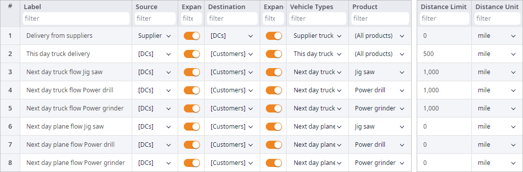
For the Next day plane vehicle type we selected the Product&distance-based cost calculator. The Distance lower limit for this policy is set to 500 miles since the lower distance deliveries will be done by the truck the day they were ordered. The Distance upper limit is set to 10000 miles as the value that cannot be reached in this scenario anyways.

Having run the Network Optimization experiment, we can observe the results.

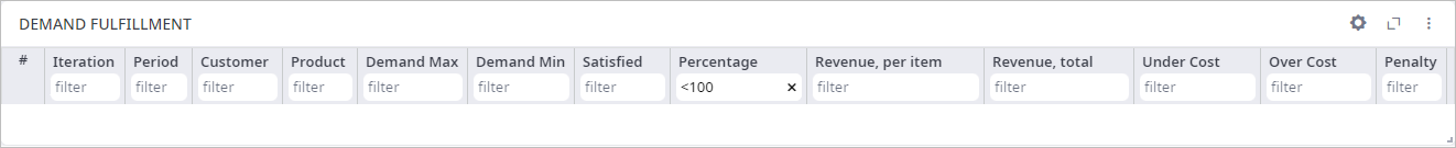
First, let us check the Demand Fulfillment table. We need to filter the Percentage column by the <100 value to see if the whole demand was fulfilled. As we can see, there are no customers with unsatisfied demand.

Now we can observe the Product Flows table to see the vehicle type used to deliver products to each of the customers.

As we can see from the Named expressions table not all demand was satisfied on the same day the products were ordered. There is still flow delivered on the second day, but the number of these deliveries is not significant.

The Travel Time value in the Product Flows table is calculated in the project time units (hours, in this case). This value is calculated just using vehicle speed and distance and drivers working hours are not considered. If the Travel Time value for the flow is greater than the daily working hours, the actual number of travel days can be calculated by dividing the value from the field by the available working hours amount.

The small amount of the next-day delivery also means that the penalty for the late delivery will be also small. We can check the penalty value in the Objective members or the Overall Stats tables of the results.

How can we improve this article?

Send