In the previous phases we created our supply chain scenario, specified customers, product, its parameters and added demand for our customers. We covered all those steps to provide the necessary information to run the Greenfield Analysis experiment.

In this phase we will configure and run the GFA (Greenfield Analysis) experiment.

Let us create GFA experiment and see what results we can get.

Create a new GFA experiment

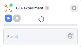
1. In the experiments section click the GFA experiment tile to open its controls.

   

2. In the expanded tile click the Show settings icon to open the experiment's settings.

   

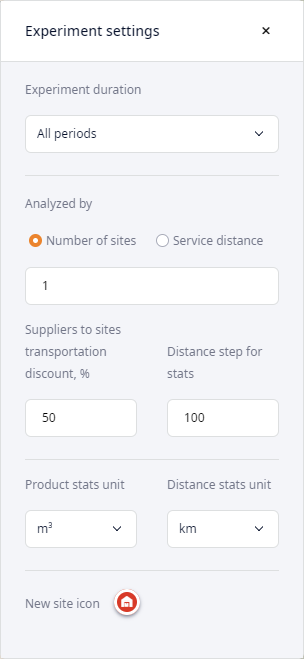
   Now we can set the experiment a task to either define the optimal quantity of DCs needed to provide our customers with a high quality service or calculate the best locations for a certain quantity of DCs.

   Since we are ready to invest into 4 distribution centers, we will start with configuring the experiment to find the optimal locations for 4 DCs.

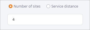
3. Set the Number of sites parameter to 4.

   

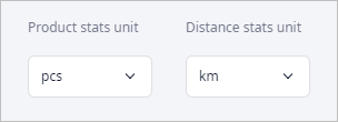
4. Set Product stats unit to pcs, since we have previously set our product to be measured in pieces.

   

5. Now run the experiment by clicking Run on the experiment's tile.

Once the experiment is completed, a new Result item will be created below the GFA experiment tile. You will be automatically taken to the new item's page containing the experiment results.

The result items can be renamed if needed. It might be useful in case of multiple experiment runs, resulting in numerous similarly named items (Result, Result 2, Result 3 ... Result 17).

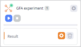
Let us take a closer look at the Result. Click the Expand map icon to hide all panels and expand the map view. You can see new elements on the GIS map. These are the distribution centers (DCs), which were created during the GFA execution. They were placed in the most advantageous locations, which were defined by the experiment considering all the data that we had provided in the previous steps of this tutorial.

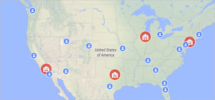
The customers and the DCs are currently not visually connected on the GIS map.

Activate paths visualization

1. Click the Show straight connections icon to visualize paths from each distribution center to each customer.

   The connections are drawn straight because the GFA experiment does not consider actual roads. Use the GFA with roads experiment if actual roads and population of the cities must be considered.

   

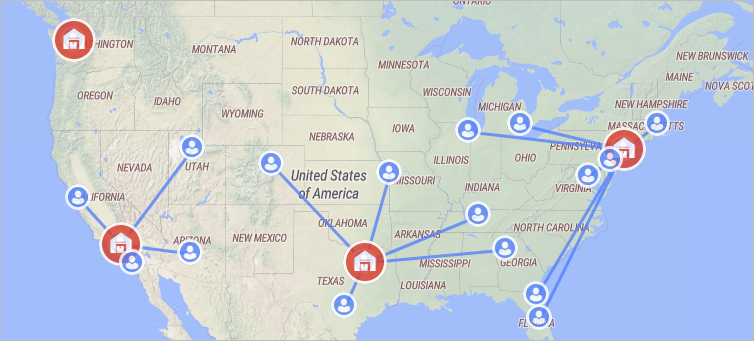
We will keep the default name of the GFA experiment result in this tutorial, but you can rename it.

Rename a result item

1. Click the Minimize map icon to show all panels.
2. Right-click the Result and select Edit.

   

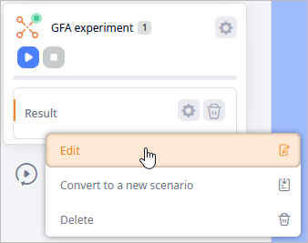
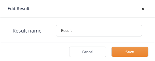
3. Type in the meaningful name reflecting the content of the experiment run (e.g. 4 DC locations to refer to the specified quantity of facilities).

   

4. Click Save to save the changes and close the dialog box. The name of the Result item will be changed to the specified one.

Now we will configure the experiment to find the optimal quantity of DCs, which could satisfy our customers' demand and at the same time maintain high level of service. To do that we must make sure that orders will be delivered in time, i.e. the DCs must not be located too far from the customers to be able to deliver the ordered product within a few days. Taking into account that customers are scattered from the east coast to the west coast, we will set the Service distance to 1000.

Modify GFA settings

1. Click GFA experiment to navigate back to the experiment's configuration page.

   

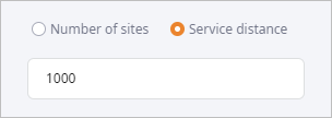
2. Click the Service distance radio button and type 1000 in the parameter's field to consider this service distance, i.e., the maximum distance between a customer and a distribution center.

   

3. Now run the experiment by clicking Run on the experiment's tile.

   You will be taken to the Result 2 item with the current experiment's results, in which anyLogistix suggests us to have 3 distribution centers.

   

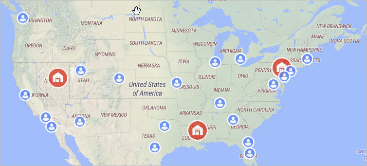
Apart from being displayed on the GIS map, the experiment results are also available in the dashboard below the experiment's view in the form of statistics distributed through the pages on the left (each page refers to a certain type of statistics). The pages contain detailed statistics on:

• Product Flows — the flows of the supply chain from the offered DC locations to the customers that we specify.
• New Site Locations — the new sites that were created as the result of the experiment.
• Distance Coverage by Demand — the distance to cover to satisfy a certain percentage of the demand.
• Demand Coverage by Distance — the demand to satisfy within a certain distance.

If required, you can rename, remove a page, or export the statistics of a page to MS Excel file.

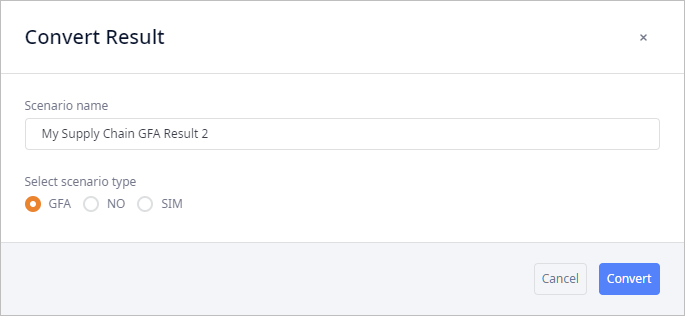
The results we received can be further used in our supply chain. We consider Result 2 offering 3 DCs to be the best solution for us. Now we need to convert it to a scenario to be able to modify it later and use it in other experiments.

Convert experiment results to a scenario

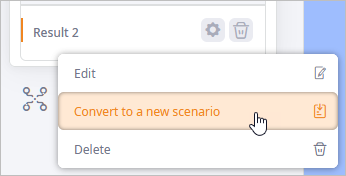
1. Right-click Result 2 item and select Convert to a new scenario.

   

2. In the opened dialog box specify new Scenario name if required, then click Convert

   

   The current results will be converted to a new scenario with its name reflecting:
   • The type of the experiment it is derived from.
   • The ordinal number of the experiment result that has been used as basis for the current scenario.

   The experiment results will not be deleted. You will be able to find them by simply switching to the original My Supply Chain scenario.

The following tables of the My Supply Chain GFA Result 2 scenario contain new data as compared to the original My Supply Chain scenario: DCs and Factories, Groups, Locations, Sourcing. Let us examine the new data.

Observe new data in tables

1. Navigate to the DCs and Factories table. This table is used to specify distribution centers and factories that comprise your supply chain. The table contains three records, one for each DC:

   • The Name column contains the names of each new facility (GFA DC ... GFA DC 3). The name consists of:
     • The name of the experiment (GFA).
     • The name of the DC (it can be DC ... DC 15, etc., depending on the resulting quantity of offered facilities).
   • The Type column specifies the type of the site. The DC type was automatically set, based on the experiment results.
   • The Location column contains the automatically created locations for each DC (detailed information on locations is available in the Locations table).
   • The Inclusion Type column defines if this or that facility will be considered by any future experiment run.
   • The Icon column defines the icon set to each object of this type. You can change icon either of a particular object, or of all objects of this type.

   

2. Now switch to the Sourcing table. The Sourcing table is used to define sourcing policies:

   • What products are shipped
   • Who the products are shipped to
   • How to choose where the products are shipped from

   In other words it shows the dependencies between warehouses and customers.

   The Sourcing table, just like the DCs and Factories table, contains the results of the GFA experiment. Let us take a closer look at the records in this table:

   • The Delivery Destination column contains groups of customers. All the specified customers have been divided into groups, one for each DC that the GFA experiment offers us to have (complete list of customers referring to this or that group is available in the Groups table).
   • The Product column specifies the product that must be shipped to the customers. The PS4 was automatically set considering the specified demand.
   • The Source column contains the sources for the specified product. In our case these are the DCs created by the GFA (the data was taken from the DCs and Factories table).

   

With the final step of converting the GFA experiment results to new scenario of GFA type we have completed GFA tutorial.

We can move on now to further use this scenario in the Network Optimization experiment.

How can we improve this article?

Send