This example model will explain the use of Custom Constraints and shadow objects in anyLogistix.

We consider a supply chain delivering diesel oil and vitroil from Kuwait to Saudi Arabia with:

• Distribution center located in Kuwait
• Transshipment base in Ras Tanura
• Customer in Yanbu

The following vehicles deliver the products throughout the supply chain:

• Pipeline (PL)
• Acid Tank Truck (ATT)
• Acid Tank Car (ATC)
• Rail Tank Car (RTC)

There are two ways to deliver the products:

• Directly to Yanbu
• Through the transshipment base in Ras Tanura

The goods from Kuwait are transported by:

• Highway transport to the Yanbu base throughout the entire year (except for the two periods of path inaccessibility).
• River barges to the Ras Tanura base during navigation period (June-September).
• Highway transport (December-March only) from Ras Tanura to the Yanbu base.

The product delivery in our supply chain consists of several stages. There is a max product flow throughput defined for each stage:

Stage	Max throughput, ton/h
Diesel fuel
Loading a vehicle	25
Sending from Kuwait	25
Transshipment in Ras Tanura	50
Sending from Ras Tanura	40
Unloading in Yanbu	33
Sulfuric Acid
Loading vehicle	40
Sending to Yanbu	28,6
Unloading in Yanbu	28,6

• Procurement strategy optimization of different products in case of the current warehouse and transport infrastructure.
• Estimate the required number of oil and acid tank trucks and barges to transfer diesel and acid on all routes.

As mentioned above, our supply chain has three nodes (DC, transshipment base, and customer). We will have to model them using three primary objects and two shadow objects, making a total of five objects.

A shadow object (DC, Supplier, etc.) is an object placed in the same location with the “primary” object. It provides supporting functions that are by default incompatible with the primary object’s type. For example, a DC cannot generate an unlimited flow of products by default, but a Supplier can, so we attach a shadow Supplier to a DC by placing it in the DC’s location.

The model will comprise the following objects:

• Product Stock — a shadow object (a Supplier object in the Kuwait location) generating a free and unlimited flow of goods to the Kuwait DC. This will free us from specifying the actual source of products for this DC, since it is not a part of the problem we are solving.
• Kuwait — Kuwait warehouse (a DC object).
• Ras Tanura — Ras Tanura transshipment base (a DC object).
• Yanbu — a shadow object (a DC object in the Yanbu Customer location) that limits the max stock of the customer warehouse, since we do not want to consider it unlimited.
• Yanbu Customer — the customer that generates demand for the products.

The supply chain will now have the following structure, with the Supplier and Customer placed in the same locations as DCs in Kuwait and Yanbu, respectively:

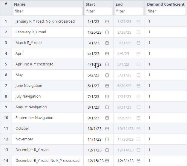
We have created 14 periods to reflect the important times in our model:

• 12 periods represent the 12 months of the simulation year. Each period has its own product flow and paths combination
• Another 2 periods will be used to define unavailability of the road at certain point in April and December

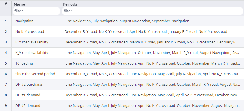
Additionally, we have defined period groups, which simplify the process of defining conditions, as we will define them for the whole group, rather than for each period individually.

To represent the flow restrictions mentioned in the table above (throughput limitations), we create Custom Constraints (CCs) for each Product Flow between the facilities within every time period. These constraints limit the time spent on performing each of the actions from the table to the time available in each period

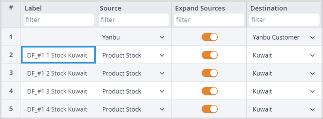
Prior to setting up CCs, we define unique labels for all records of the Product Flows table, to be able to reference them later in the CC expressions. Each flow label contains references to product, period number, source, and destination of this particular flow.

For example, the label of the second record DF_#1 1 Stock Kuwait says that this flow is defined for the DF_#1 product, which is transported within the period 1 (2022-01-01 — 2022-01-25) from the Product Stock to Kuwait (Stock Kuwait).

The first record does not require any label, since it will not be used in any CC. This flow represents the process of transferring the products from the shadow DC object to the demanding customer

Here's how the constraint for the Sulfuric Acid product is defined:

The left-hand side of the constraint holds the expression estimating the time required to perform the action, for which this constraint is created (“Loading a vehicle”, that is, transferring the product from the Product Stock to the Kuwait DC). This value is calculated as the product flow divided by the throughput of this action, where:

• Product flow — the actual product flow value. We are using the SA 1 Stock Kuwait label from the Product Flows table to refer to the flow value).
• The throughput value — 1 / 40 = 0.025, which allows us to use multiplication in the expression. The value of 40 ton/h is taken from the table above (see the Loading vehicle record of the Sulfuric Acid section)

In the same way we estimate the time for each action, and define constraints with the received data.

The right-hand side of the constraint holds the length of the period in hours (defined in the Periods table) this action refers to. For example, the length of the first period is 25 days, or 600 hours. That is why in the example above we put 600, which limits the maximum time spent on performing this action.
In this model, we use two equivalent options of defining the constraints of hours available. We may do either of the following:

• Define the whole restriction in one constraint.
• Introduce a new variable and define an expression for it in the first line.
  Then use this variable to set a restriction in the second line.

The received results show that to satisfy the demand of the customer for the DF_#1 product when the Kuwait-Yanbu path is inaccessible, the product delivery proceeds from the Ras Tanura transshipment base. But because delivering to Ras Tanura is only available in navigation periods (June — September), the required amount of DF_#1 is stored in Ras Tanura from September to December, when highway path from Ras Tanura to Yanbu becomes available.

The estimated number of vehicles, considering the given restrictions and capacities, can be seen in the Vehicle Flows table. For example, since capacity of the pipeline is set to 1 ton, the number of vehicle trips is equal to the total product flow for every month (in tons).

How can we improve this article?

Send