In this example, we will learn how to vary demand using the demand coefficient or to define stochastic demand to make the supply chain closer to reality. Also, we will configure and use the Variation experiment to easier checking the difference between the values of the demand coefficient.
This scenario is a part of the sequence of 4 example models that illustrate the different stages of supply chain analysis:
- GFA US Distribution Network — a scenario for finding locations for warehouses. This is the scenario we will investigate now.
- NO US Distribution Network — a scenario for selecting facilities from the suggested list of distribution centers and ports.
- SIM Distribution Network Analysis — scenario that is based on the result of the optimization. This result has been converted to the SIM scenario to analyze the suggested network in more detail.
- SIM Budget Comparison — a scenario for analyzing the impact of unstable demand on the service level of the supply chain.
All input data can be found in the previous examples of this sequence.
In the previous step, we converted the result of network optimization into a SIM scenario and conducted a simulation experiment. After that, we analyzed statistics and decided to update the scenario using a Safety stock estimation experiment to get a better service level.
anyLogistix offers two scenarios:
- Example with estimated demand without variation.
- Example with triangular demand distribution and with demand variation (in Variation experiment).
In the second scenario, we can see how the randomness of demand can be implemented to reflect the real life. Here we use the triangular distribution to add stochastics to the scenario.
- Run Simulation experiments for both offered scenarios and compare results.
- Check Service Level statistics for different demand coefficients using Variation experiment.
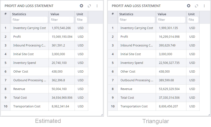
Let us run a Simulation experiment for both scenarios and analyze received statistics. We can review each network budgeting detail for both scenarios. Financial statistics are available on the Profit and Loss Statement page of the experiment results.

As we can see, in case of the triangular demand distribution the amount of demand is higher than estimated. So, revenue, profit, and all the costs, that depend on the amount of delivered products, increase correspondingly.
For the scenario with estimated demand, we can also change all the demand values at once, by using the demand coefficient in the Periods table. For example, if we set the demand coefficient to 1.2 for a period, the demand of all customers will increase by 20%.
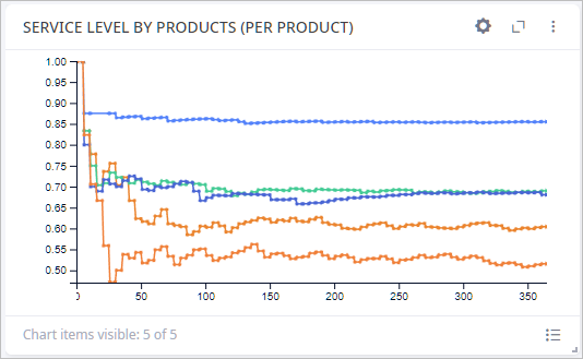
We can observe the result of the Simulation experiment to understand the impact of this change in input data. In the Service Level tab, we can see, that there is a shortage of products to ship to the customers.

To easily compare service levels for different values of demand coefficient, we can use the Variation experiment.
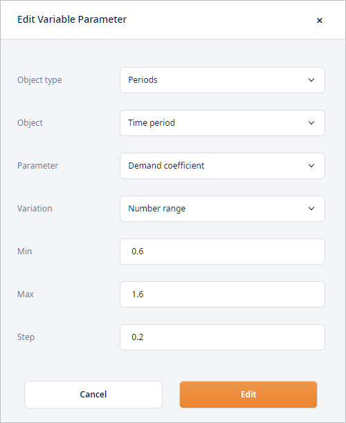
Open the Variation experiment settings for the Triangular Demand Distribution scenario. Here we can see that the variable parameter is already defined, but we can go and check details by selecting it and clicking the Edit button. On the image below we define the right parameter that we want to variate, and the way it will be iterated. So, the demand coefficient will increase by 0.2 every iteration of the experiment starting from 0.6 and ending with 1.6.

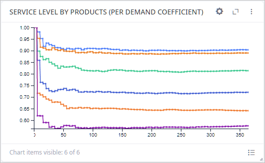
Also, we add the Service Level by Products chart (per demand coefficient) onto the dashboard to visually compare the results of the Variation experiment.
Run the variation experiment. The result shows that by increasing the demand coefficient the profit and the total cost increase as well, but the service level is decreasing to the inappropriate values.


As we can see, the supply chain defined in this scenario doesn't show good performance if the demand coefficient increases. The goal of the manager would be to find a solution to address this issue. You could try to either optimize the parameters of the inventory policies, or find the best combination of them .
-
How can we improve this article?
-

