To complete this tutorial, you must work with a scenario that contains at least the following:

• Customers
• Product(s)
• Demand
• Distribution centers
• Supplier

In this phase of the tutorial we will complete the following steps after creating NO type scenario.

• Define alternative distribution center locations.
• Set inclusion type for the supply chain's distribution centers
• Create groups of alternative distribution centers locations per servicing area and:
  • Specify them as sources in the Products Flows table.
  • Define storage policies in the Product Storages table.
• Define assets constraints to set experiment's objective.
• Add a supplier (obligatory to run the NO experiment) and configure it.
• Adjust cost calculation policy parameters.
• And finally run the experiment.

To create a scenario to work with, you can either instantly download and import the My Supply Chain GFA Result 2 scenario, which is based on the result of the GFA experiment, or you can provide your own scenario data that you would like to optimize with the help of the Network Optimization experiment.

We will use the GFA scenario containing experiment results as the basis for our Network Optimization experiment tutorial.

The numbered lists in tutorials are actually checklists. Click the numbers to save your progress!

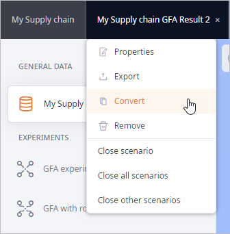
Convert scenario from GFA type to NO type

1. Right click the My Supply Chain GFA Result 2 scenario and select the Convert option.

   

2. In the opened dialog box select the NO radio button of the Select scenario type parameter.

   The name of the scenario may seem quite long. If required you can rename it now or later by right-clicking the new copy and selecting Properties from the context menu, and then specifying the desired name in the Scenario name field.

3. Click Convert. You will be taken to the Network Optimization tab containing the just created copy.

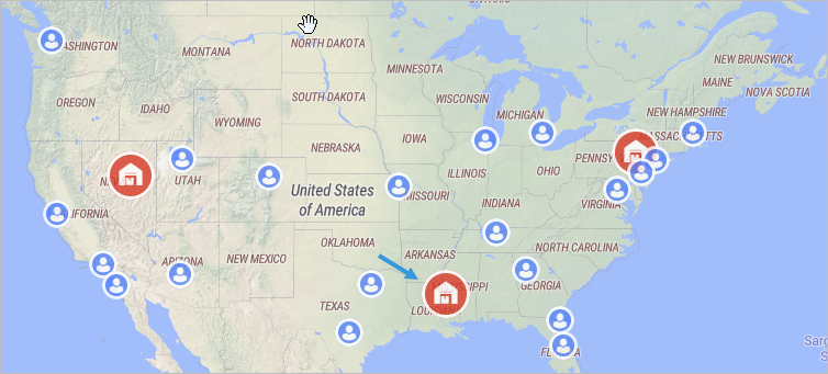
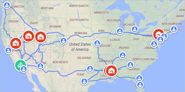
Let us have a closer look at the scenario's data. GFA executed rough calculation of distribution center locations. It did not consider roads, cities, peculiarities of geographical areas, etc. We need to analyze the current locations and find the best locations considering the existing infrastructure.

First, we should zoom in to see if the distribution centers are placed in the advantageous spots with easy access to highways. Depending on the remoteness of a distribution center from the required infrastructure we will either move it towards the nearest city/highway or specify a number of potentially interesting locations for it. The best locations will be found by the Network Optimization experiment.

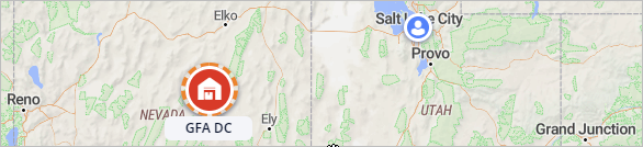
Let us now examine the locations offered by the GFA experiment. We shall start with the distribution center in the middle.

Check distribution center location

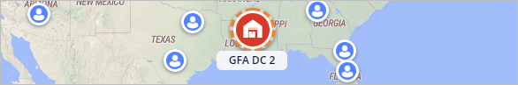
1. Click the distribution center on the GIS map. A tooltip will appear providing information on the selected distribution center.

   

2. Zoom in by scrolling your mouse wheel. Place your mouse cursor over the GFA DC 2 to center the map while zooming in.
   You will see that it is located too far from the closest highway/city. We will have to find a better location for this distribution center.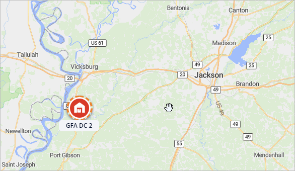

   

Since we cannot tell where exactly to place this particular distribution center due to its initial location, we should define several potential locations, which would meet our requirements. These locations will be further used by the Network Optimization experiment, which will try to find the optimal location (or locations, depending on the set parameters) for this distribution center.

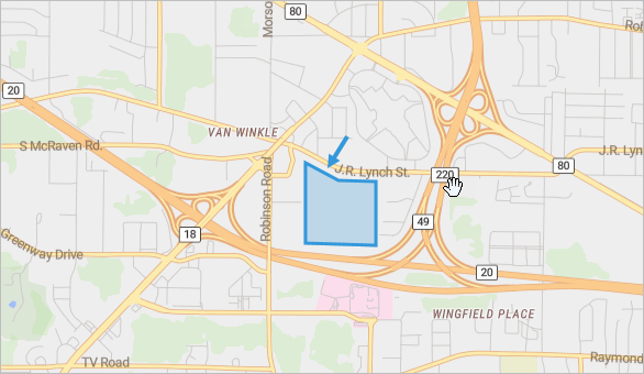
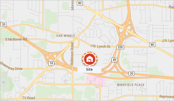
Let us consider Jackson and Vicksburg cities as potential GFA DC 2 locations.

Define potential locations

1. Zoom in to Jackson city close enough to search for the potential location somewhere near an intersection involving Interstate 20.

   The area with numerous intersections seems prospective. We will place a distribution center here to further consider this location in the experiment.

   

2. Click the Create distribution center icon in the GIS map toolbar and click somewhere within the area to place a distribution center.

   

3. When done, click the Panning mode icon in the toolbar to exit the editing mode.
   Now let us navigate to the Vicksburg city to find alternative potential location there.
4. Zoom in and place distribution center near the Iowa Boulevard and Route 61 as shown on the screenshot below.

   

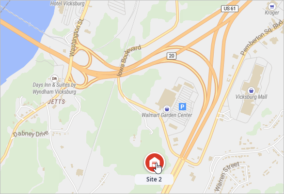
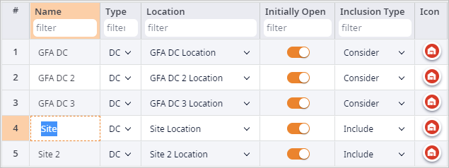
We have set two potential locations for the GFA DC 2 warehouse, now we must give them meaningful names that would reflect their locations. Let us name them Jackson DC and Vicksburg DC correspondingly.

Rename the distribution centers

1. Navigate to the Distribution Centers table (it is currently open below the GIS map). The table contains five records, one for each distribution center (three distribution centers offered by the GFA experiment, plus two that we have just defined).

   

2. Double-click the Distribution center field in the Name column to activate the editing mode.

   

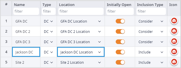
3. Type in Jackson DC and press Enter to exit the editing mode. The name of the distribution center will be changed, its Location name will be automatically updated.

   

4. In the same way rename the Distribution center 2 object to Vicksburg DC.

   

Now we will move on and check locations of the other two distribution centers. Let us continue with the distribution center in the western part of the United States.

Check distribution center location

1. Click the leftmost distribution center on the GIS map. A tooltip will appear providing information about it.

   

2. Place mouse cursor over the GFA DC to center the map while zooming in. Scroll mouse wheel to zoom in.
   You will see that it is located too far from the closest highway/city. We will have to find a better location for this distribution center.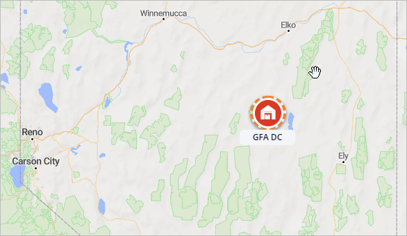

   

   As we can see this distribution center is not in the most popular place either. We will consider Carson City, Elko and West valley city (located in the suburb of the Salt Lake City) as potential GFA DC locations.

Define potential locations

1. Zoom in to Elko city close enough to search for the potential location somewhere near the railroad.
   The area shown on the screenshot below seems prospective. We will place a distribution center here to further consider this location in the experiment.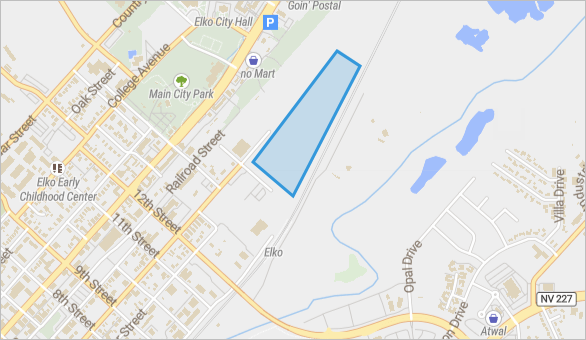

   

2. Click the Create distribution center icon in the toolbar of the GIS map view and click somewhere within the area to place a distribution center.

   

3. When done, click the Panning mode icon in the toolbar to exit the editing mode.
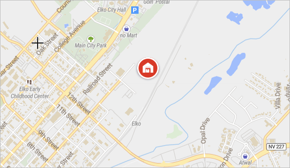
4. Rename the created Distribution center to Elko DC in the Distribution Centers table below the GIS map.
   Now let us navigate to the Carson City to find alternative potential location there.
5. Zoom in and place a distribution center near the East 5th St as shown on the screenshot below.

   

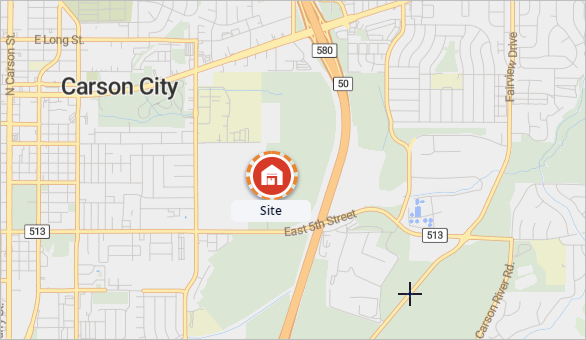
6. Rename the created Distribution center to Carson City DC in the Distribution Centers table.
7. Now zoom in to the West Valley City and place a distribution center in the potential location as shown on the screenshot below.

   

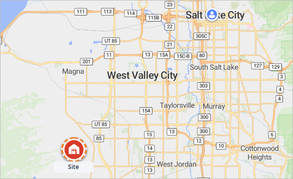
8. Rename the created distribution center to West Valley City DC in the Distribution Centers table.

We have set three potential locations for the GFA DC warehouse and we may finally move on to the third distribution center proposed by the GFA experiment. It is located in the eastern part of the United States.

Check distribution center location

1. Click the distribution center on the GIS map. A tooltip will appear providing information on the selected distribution center.

   

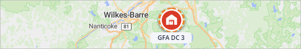
2. Zoom in by scrolling your mouse wheel. Place mouse cursor over the GFA DC 3 to center the map while zooming in.
   You will see that GFA DC 3 is located on the State Game Lands, which is the reason why it must be moved. Wilkes-Barre city to the West is the nearest large city. If we look closer at it, we will see that it is a good location with numerous PA routes, Interstate highway 81, and Wilkes-Barre/Scranton International Airport.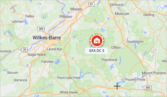

   

Since Wilkes-Barre is located in just 14 kilometers from the current distribution center location, we will simply move this distribution center towards the Wilkes-Barre's environs.

Adjust location of the distribution center

1. Zoom into the Wilkes-Barre city area close enough to see its streets and potentially prospective locations somewhere near the highways.
   There is a vast piece of land right next to the city with easy access to the intersection involving Interstate 81 with PA 309 and PA 115 routes.

   

2. Zoom out, click GFA DC 3 and drag it to this area.

   

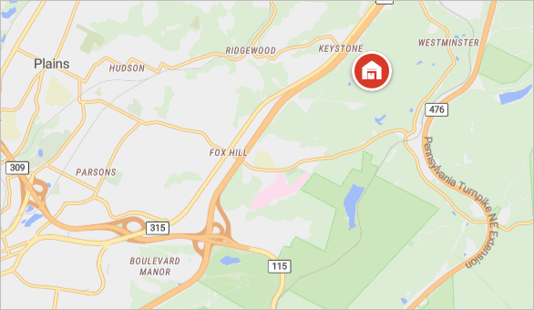
3. We have relocated GFA DC 3 and now we must give it a meaningful name that would reflect its location. Let us name it Wilkes-Barre DC.

At last we have completed setting up the potential distribution centers locations. You may zoom out now to observe the whole picture.

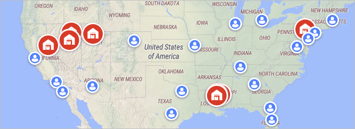
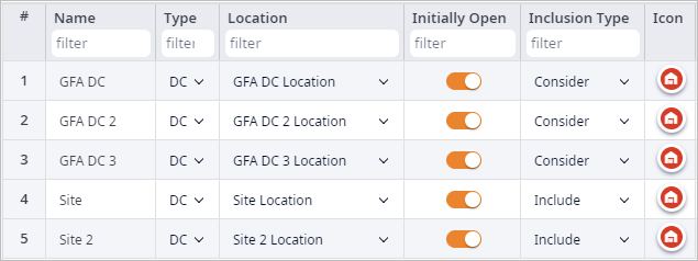
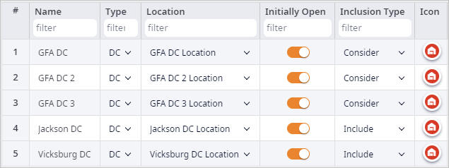
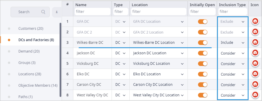
The GIS map currently shows the total of 8 distribution centers. Here belong the three distribution centers that were taken from the GFA result, and the five distribution centers that we have just created while defining the potential locations. By default all these distribution centers are included in the Network Optimization experiment. If you navigate to the Distribution Centers table, you will see the distribution centers and their types of inclusion.

Above the line you can see the distribution centers, which were initially present in this scenario. Below the line you can see all the distribution centers that we have just created.

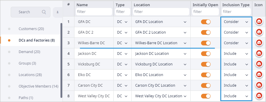
Now we need to specify the inclusion type for each distribution center. We will assign the following inclusion types:

• Wilkes-Barre DC — Include. The experiment will keep the current distribution center in the supply chain configuration.
• GFA DC — Exclude. The distribution center will not be considered by the experiment.
• GFA DC 2 — Exclude.The distribution center will not be considered by the experiment.
• Jackson DC ... West Valley City DC — Consider. The experiment will consider these distribution centers to find the best solution among them.

Change the inclusion type of a distribution center

1. Select the GFA DC and GFA DC 2 cells in the Inclusion Type column by Ctrl clicking them.
2. Press Spacebar to open a pop-up window with a drop-down list of inclusion types.
3. Select Exclude and click OK.

   Once you have marked the GFA DC and GFA DC 2 as "Excluded", the table records will be grayed out and the corresponding facilities will disappear from the GIS map.

   

4. In the same way mark the distribution centers that we have added to our model (Jackson DC ... West Valley City DC) as “Consider”. You may select a number of successive cells by Shift + clicking the first and the last cells.

In the end your Inclusion Type column must look like this:

We have successfully defined alternative locations. Now, to make the Network Optimization experiment choose the best distribution center locations among the defined ones, we will create a condition in the Assets Constraints table. We will also specify the final number of distribution centers that we want the experiment to find.

Since the distribution centers we want the experiment to choose from refer to two different locations with two independent groups of customers, we must first create two groups of alternative locations the experiment will work with.

Create groups of alternative locations

1. Navigate to the Groups table. You will see that it already contains a number of automatically created groups.
   Judging from the names of the groups we can see that they were created based on the result of the GFA experiment.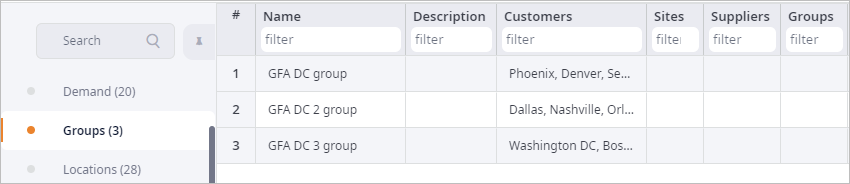

   

2. Click Add below the table to create a new group. A new table record named Group will be created.

   

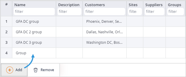
3. Double-click the Group cell and type in GFA DC alternatives to specify the name of the group.

We have created and renamed a new group. Now we need to define the content of the group. We know that this group will contain distribution centers. The distribution centers we need can be defined in the Sites column of this table.

Define distribution centers for the group

1. Double-click the GFA DC alternatives row cell in the Sites column. A dialog box will open containing all the available distribution centers to choose from.

   

2. Click the toggle buttons in the Included column referring to the Elko DC, Carson City DC and West Valley City DC.

   

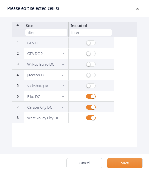
3. Click Save to close the dialog box and apply the changes.

   

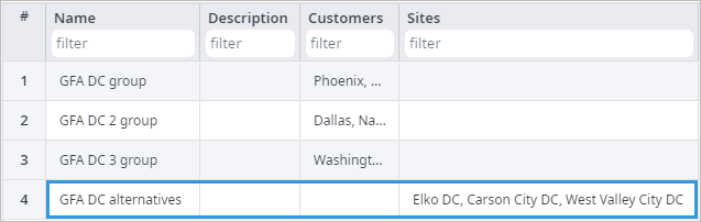
4. In the same way create the GFA DC 2 alternatives group that will contain Jackson DC and Vicksburg DC.

Now we can proceed to creating a condition that will be used by the Network Optimization experiment.

Create condition optimizing distribution centers locations

1. Navigate to the Assets Constraints table and click Add to create a new table record.
2. Click the Group cell to open a drop-down list of available groups and select the GFA DC alternatives group. In such a way we tell the experiment to choose among the distribution centers from this group.
3. Specify the required number of distribution centers that the experiment must choose:
   • Click the Min cell and type in 1.
   • Click the Max cell and type in 1.
4. In the same way create the second record for the GFA DC 2 alternatives group.
   Your Assets Constraints table should look like this.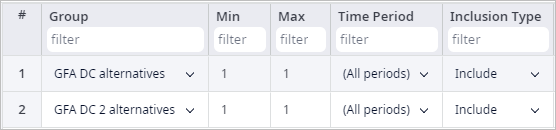

   

We have set the alternative distribution centers locations and defined conditions for the Network Optimization experiment to work with.

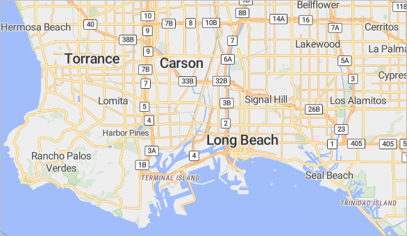
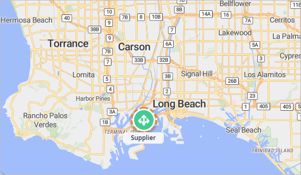
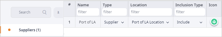
Please note that It is obligatory to have a supplier to run the NO experiment. We currently have no supplier. Let us place it in the port of Los Angeles, which also happens to be the busiest US port.

Add a PS4 Supplier

1. Click the GIS map to activate it and zoom in to the Port of Los Angeles, located right next to the Long Beach.

   

2. Click the Create supplier icon in the toolbar menu of the GIS map and click the port area to place the supplier.
   

   

3. When done, click the Panning mode icon.

We have added Sony PS4 supplier, which will provide our distribution centers with the consoles and now we need to configure it within our supply chain.

Configure supplier

1. Navigate to the Suppliers table below the GIS map and name it Port of LA.

   

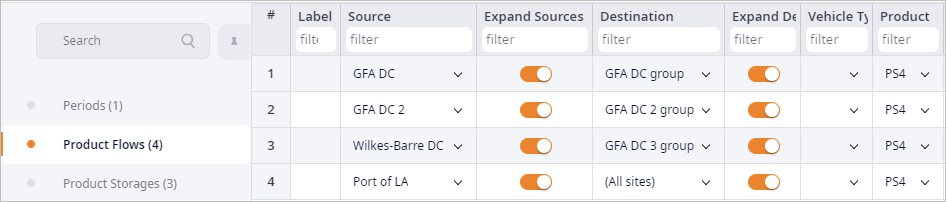
2. Navigate to the Product Flows table and create a new flow of products from the supplier to the distribution centers:
   • Click Add to create a new record.
   • Double-click the cell in the Source column and select Port of LA from the drop-down list.
   • Double-click the cell in the Destination column and select All sites from the drop-down list.
   • In the same way specify PS4 in the Product column cell.

When done, the Product Flows table should look like this:

• Sources #1-3 are the ones that were automatically created on converting the GFA experiment result to the scenario.
• The source #4 is the one with the supplier.

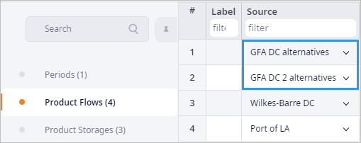
As you remember we have previously created two groups containing alternative distribution centers locations, which must be considered by the NO experiment. We need to:

• Set those groups as product sources
• Define product storage policy for those groups

Let us start with defining the sources, since we are in the Product Flows table already.

Configure product sources

1. Double-click GFA DC and select GFA DC alternatives from the drop-down list of available sources.
2. Double-click GFA DC 2 and select GFA DC 2 alternatives from the drop-down list of available sources.

   

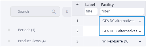
Now move on to the Product Storages table to define the storage policies.

Define storage policies

1. Navigate to the Product Storages table.
2. Double-click GFA DC and select GFA DC alternatives from the drop-down list of available sources.
3. Double-click GFA DC 2 and select GFA DC 2 alternatives from the drop-down list of available sources.

   When done, the Product Storages table should look like this:

   

The last thing to do before running the experiment is to modify the parameters of the Cost Calculation policy, which can be found in the Paths table. The changes will affect the product measurement unit type (it must correspond to the one specified in the Unit column of the Products table) and the transportation cost of the specified measurement unit type.

Modify Cost Calculation policy

1. In the Paths table double-click the cell of the Cost Calculation Parameters column.
   A dialog box will open allowing you to modify the policy parameters.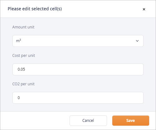

   

2. Click the Amount unit drop-down list and select pcs.
3. Now click the Cost per unit field and type in 0.002, which is the cost of transportation of one PS4 unit in a standard 20ft truck.

   

Finally, make sure that the vehicle's capacity is measured in the product units (pcs).

Define vehicle capacity units

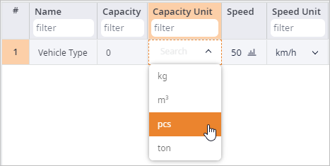
1. Open the Vehicle Types table. You will see that the table contains the default vehicle type, which was created on converting the GFA scenario to NO scenario.

   

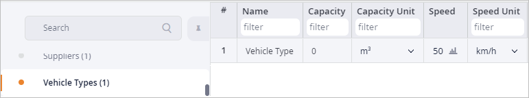
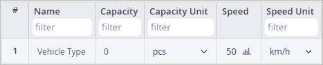
2. Double-click the cell in the Capacity Unit column and select pcs from the drop-down list.

   

   When done, the table should look like this

   

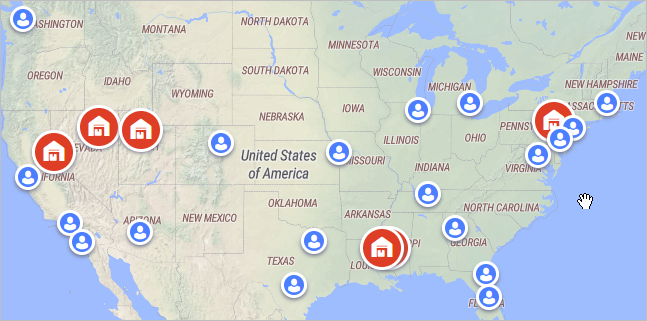
If you enable connections on the GIS map, you will see the paths from each distribution center to each customer. The actual routes are used by default in anyLogistix.

Enable paths on the map

1. Click the Show connections button in the map toolbar to see the paths.
   The paths will be depicted as straight lines. Let anyLogistix download the data. This may take some time depending on the internet connection speed and the number of routes. Once anyLogistix applies the downloaded information to our map, we will be able to see the actual routes, which connect customers to each distribution center. The GIS map sourcing paths will change their shape in accordance with the available roads leading from the warehouses to the customers.

   Now we can see the actual roads, which will be used in our supply chain to deliver the products. If needed, we can zoom in the map to observe every route and adjust the location of a warehouse. The route will be instantly recalculated according to the new warehouse location.

That's it. We are ready to run Network Optimization. Let us create the experiment and examine the results.

Set up and run Network Optimization experiment

1. Navigate to the Experiments section and click the Network Optimization tile.
   You will be taken to the NO experiment's view with its default settings.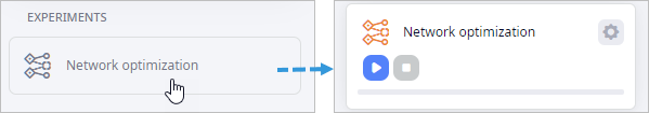

   

2. In the expanded tile click the Show settings icon to open the experiment's settings.
3. Set Number of best solutions to find to 10.

   

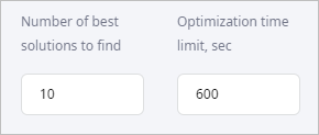
4. Set Product stats unit to pcs (it must correspond to the unit specified in the Products table).
5. Now run the experiment by clicking Run on the experiment's tile. anyLogistix will start downloading the routes for all the combinations of customers and distribution centers. Once all the routes are cached, the experiment will be executed.

Once the experiment is completed, the Result sub-item will be created below the Network Optimization tile. You will be instantly taken to it.

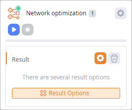
The result of the experiment will be available in the Iterations panel next to the experiment settings. This panel lists all the possible options in form of iterations cards.

The top option is the best one found during the optimization in terms of transportation costs (specified in the Paths table).

All other pages in the dashboard below the map contain additional information on the received results in the form of statistics (each page refers to a certain type of statistics).

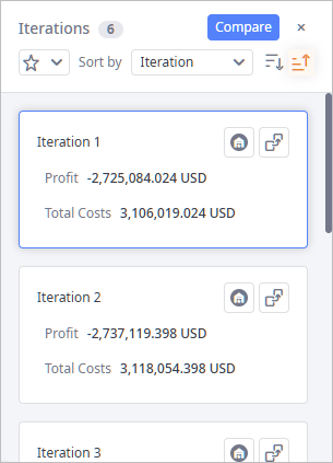
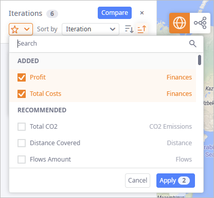
By default the iteration cards contain only Profit and Total Costs statistics. If required, you can add other metrics by clicking the icon in the header of the panel, selecting the checkboxes of the required metrics from the Recommended section of the drop-down list, and then clicking Apply.

The drop-down list contains statistics that are enabled in the Statistics Configuration dashboard.

The results of the experiment can be visually observed on the GIS map. We will also visualize routes for all sites.

1. The top iteration card is selected by default, and its solution is displayed on the GIS map.

   To see the paths, click the Show connections button in the map toolbar.

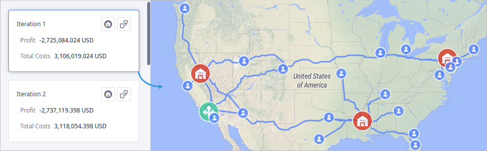
We have received the basic Network Optimization results with real routes and exact distribution centers locations.

Now we can move on to specify the price of the product, the cost of opening a warehouse and the cost of processing the outgoing shipments.

How can we improve this article?

Send