In this example, we will use the Last Mile Optimization experiment to optimize transportation routes in our supply chain by solving the Capacitated Vehicle Routing Problem with Time Windows (CVRPTW).

A company transporting flowers in the Netherlands wants to improve the efficiency of its supply chain by implementing a process for solving the analytical task of scheduling deliveries with time windows and limited vehicle capacity.

We are analyzing completed deliveries (that are based on historical data) to demonstrate how delivery network optimization may improve the outcome.

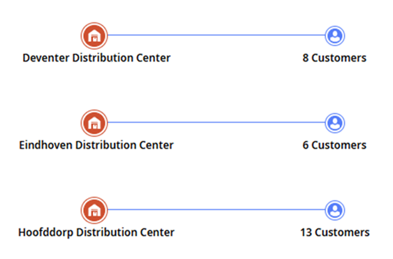
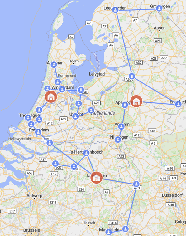
A total of 27 customers from different cities of the Netherlands were registered for the considered period.

The objects of the supply chain are not available 24/7. Both sites and certain customers have time windows that may affect order completion.

The company has 3 distribution centers, from which deliveries are made. The fleet of each distribution center has two vehicles types with different capacities and speeds.

For this task, we will assume that it takes from 10 to 15 minutes to load a vehicle at the warehouse.

Obtain an optimal shipment schedule considering delivery time, traveled distance, as well as loading and unloading times.

Create the required scenario by following the steps below:

• Define customers' demand (of historic type) in the Demand table. Each customer generates demand on daily basis daily within the period of 3-4 days.
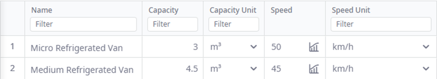
• Create two vehicle types:

  

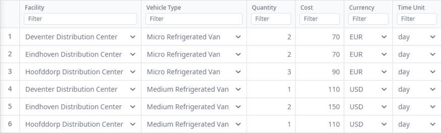
• In the Fleets table create fleets for the distribution centers (one for each vehicle type):

  

• Add necessary paths (in the Paths table) between all objects to allow the vehicles to move not only between the distribution centers and customers but also between the customers. These paths will be used for optimization.
• Add time windows for the customers (in the Time Windows table), during which they are ready to accept orders.
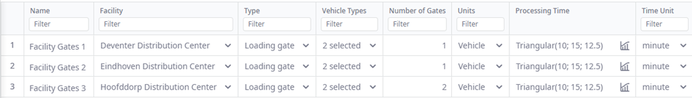
• Add loading and unloading gates (in the Loading and Unloading Gates table) to model the vehicles loading and unloading processes. To simulate the stochastic nature of loading time, we use triangular distribution:

  

Let us run the Simulation experiment and examine the received results on the KPI metrics:

We can see fulfillment of all orders, and the transportation costs according to the specified calculation policies. Additional statistics pages provide a more detailed overview of the received results.

To demonstrate unorganized deliveries without centralized planning (if we can ship it, we ship it) the LTL shipping policy was used in the Shipping table. As a result the couriers would fetch just 1 order for the delivery most of the time, and then wait at the customer's location for the availability hours defined in the Time Windows table.

Last Mile Optimization essentially implements the CVRPTW problem, which comprises:

• Objects of customer and distribution center types.
• Demand generated by the the customers (individual orders for specific product in certain amount).
• Operating hours (defined in the Time Windows table) for distribution center / customer operations.
• Vehicles have limited capacity.
• Various business constraints, such as mandatory return to the distribution center, maximum vehicle idle time, etc.
• The goal is to obtain milk runs for each vehicle type that would meet the following requirements:
  • An order can be fulfilled just once.
  • Vehicle capacity constraints are not violated.
  • The defined operating hours are not violated.
  • The total travel time is minimized.

The Last mile optimization experiment settings allow us to define:

• The planning horizon (experiment duration).
• Vehicle types that will be used by the optimizer (the optimal vehicles will be eventually used to deliver specific sets of orders in a single trip).
• Maximum shipment duration.
• Maximum vehicle idle time.
• If the vehicles should return back to the positioning site.
• etc.

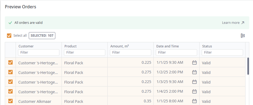
The Preview Orders table suggests that all orders that have been generated based on the scenario data and experiment parameters should be taken as the input data for the optimizer:

Let us run the experiment. The following result will be obtained within 60 seconds, since this time is allotted to the experiment by the Optimization time limit parameter:

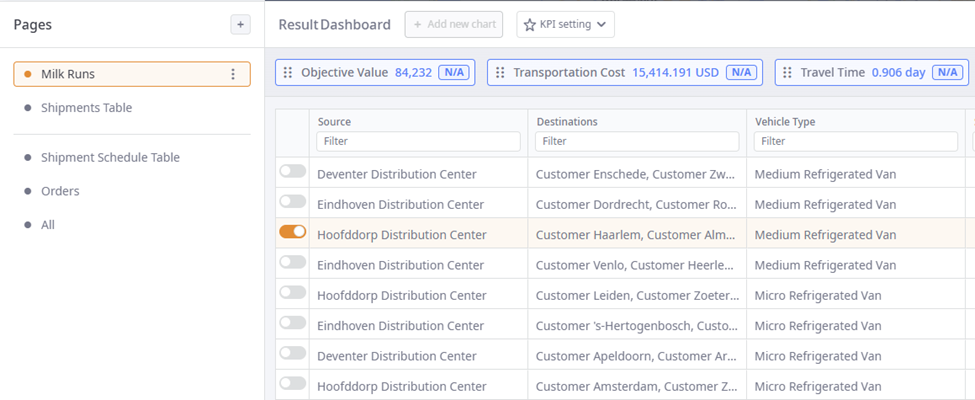
The Milk Runs dashboard page contains the list of generated milk runs with the optimized delivery times. Each milk run is a route comprising a set of customers that will be visited by a vehicle to deliver the demanded orders. On delivering the order to the last customer of a milk run, the vehicle will disappear, since the Return vehicles back to site option is not selected.

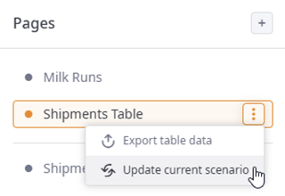
The obtained results can be applied to the current scenario. We will update the current scenario with data from the Shipments Table dashboard page by selecting the Update current scenario option from the Actions drop-down list with the Keep the current structure setting enabled in the Update Current Scenario dialog box:

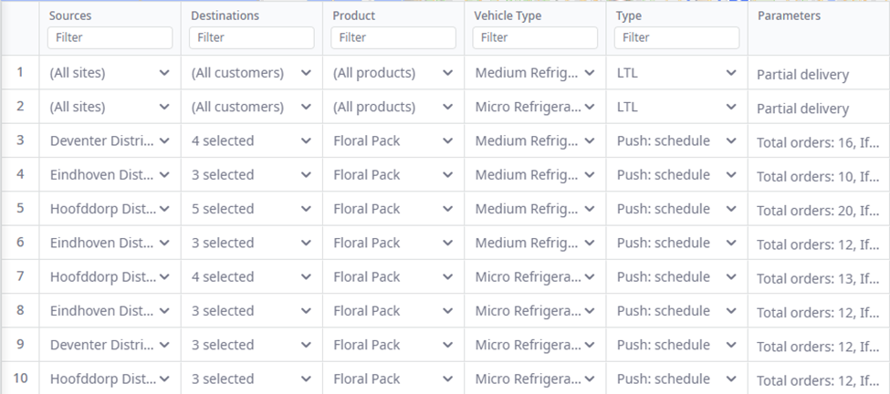
The entire structure of shipments, vehicles' loading and unloading will be added to the Shipping table of the current scenario:

The records with the old LTL policies must be removed (or excluded by setting the corresponding Inclusion Type) to ensure that all shipments will adhere to the obtained schedule only.

If we run the simulation experiment again, we will see the following changes:

In this experiment run, the Shipments dashboard page shows the history of all orders. The optimizer adjusted the shipment schedule so that each vehicle delivers as many orders as possible in one trip, which minimizes the total traveled distance decreasing it by almost 90% as compared to the original version.

The vehicles now align with the customers' order acceptance schedules, and depart only when the customer is ready to accept the order. By the time the vehicle reaches the first customer, another customer from the milk run will be ready to accept the delivery. This creates milk runs, which allows to load a vehicle with multiple orders for different customers and deliver them all within one shipment. Each generated milk run can be observed on the Milk Runs page of the obtained Last Mile Optimization experiment result:

The Last Mile Optimization experiment significantly improves delivery efficiency by planning the delivery routes considering time windows and fleet constraints.

Unlike scenarios with uncontrolled deliveries, this optimization approach:

• Reduces the total distance to travel by consolidating orders into shipments per milk run.
• Increases vehicle load rates, minimizes empty runs.
• Decreases logistics costs by ensuring better resource allocation.
• Allows importing data from the found solutions into the original scenario for further supply chain analysis.

The Last mile optimization experiment becomes a powerful tool for urban logistics planning, especially during an order surge and strict time constraints. Its application allows you to make data-driven decisions on daily basis and easily scale this approach to other regions or time horizons.

How can we improve this article?

Send