In this example, we will:

• Examine the capabilities of production modeling considering resource competition within a simulation experiment.
• Design a multi-level production schedule.
• Analyze approaches to minimizing changeover costs within a non-batch production process.

A major solar panel manufacturer in Spain sources components from France and Portugal for subsequent multi-level production at its factory. It is necessary to develop a model that satisfies the business constraints, aims at optimizing production costs and profit, and generates a complete production schedule across all levels — from components to the final product.

• The factory is located in Toledo, Spain.
• 37 customers generate periodic demand for solar panels of various types.
• Two component suppliers are based in France and Portugal.
• All panel components are produced on dedicated intermediate assembly lines.
• Solar panels of different types are produced on the final assembly lines.
• Line changeovers on the final assembly lines (from one panel type to another) require time and incur certain costs for the manufacturer.
• The factory cannot afford batch production of panels, however, panel components have their own safety stock and are replenished on a regular basis.

We will model random demand aligned with historical data. The period will be defined by the uniform distribution (14;21), and the demand will be defined by the triangular distribution (9,20,16). The scenario will contain three product types: first-level components, modular components, and final products. The production process comprises several steps. All steps are done at a single factory. First-level components are delivered to the factory on demand from the corresponding supplier.

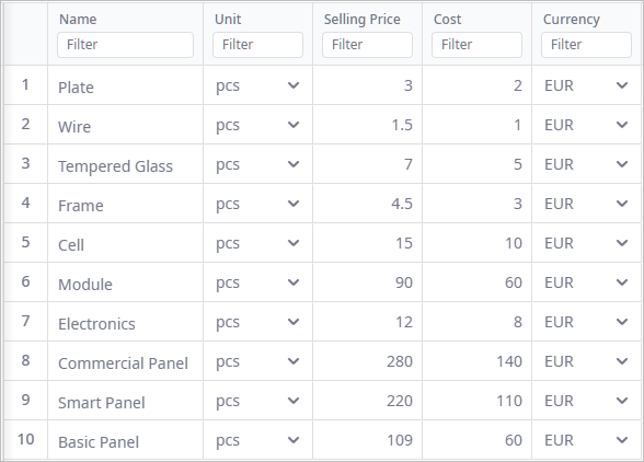
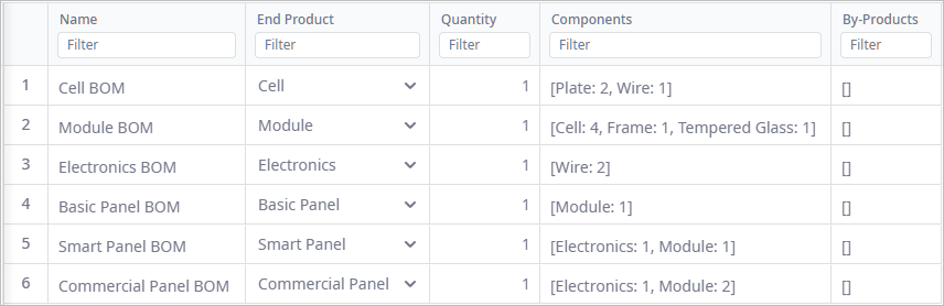
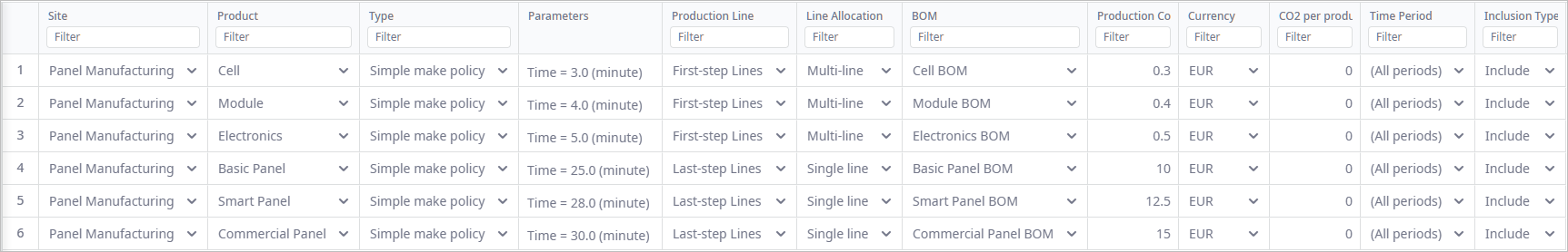
In the BOM table we will define the components and their quantities needed to produce the end products.

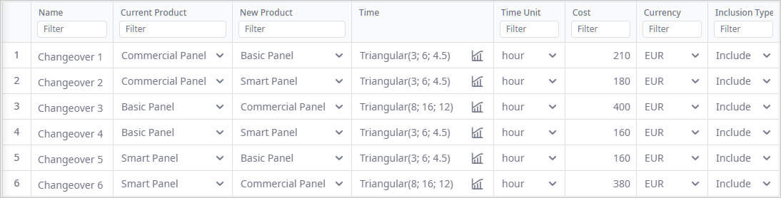
The time required to set up lines for other products will be defined in the Production Changeovers table. Switching from one product to another will require the line to:

• Become idle for a certain amount of time (defined by the triangular distribution).
• incur associated expenses, determined by the manufacturer.

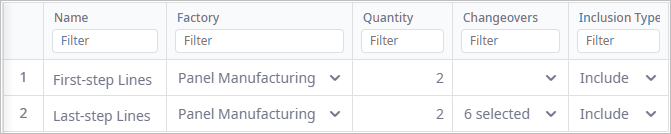
We will simulate the production of different product types on the same lines using the Production Lines table. The factory will have two types of production lines:

• First-step Lines — these 2 lines will be producing modular components.
• Last-step Lines — these 2 lines will be producing three types of panels. The defined changeover times will be applied here for switching between product types to produce.

The final production settings take into account the product that the specific line is currently producing, the BOM that is used to produce this product, and the time it takes to produce the product. The production time of each order changes proportionally to the number of involved lines (defined by the Line Allocation parameter). In our case, each production order can be assigned to one of the two available lines, meaning that the factory can produce a maximum of two orders simultaneously. Modular components, on the other hand, can utilize all available lines for each order due to the faster and simplified assembly process.

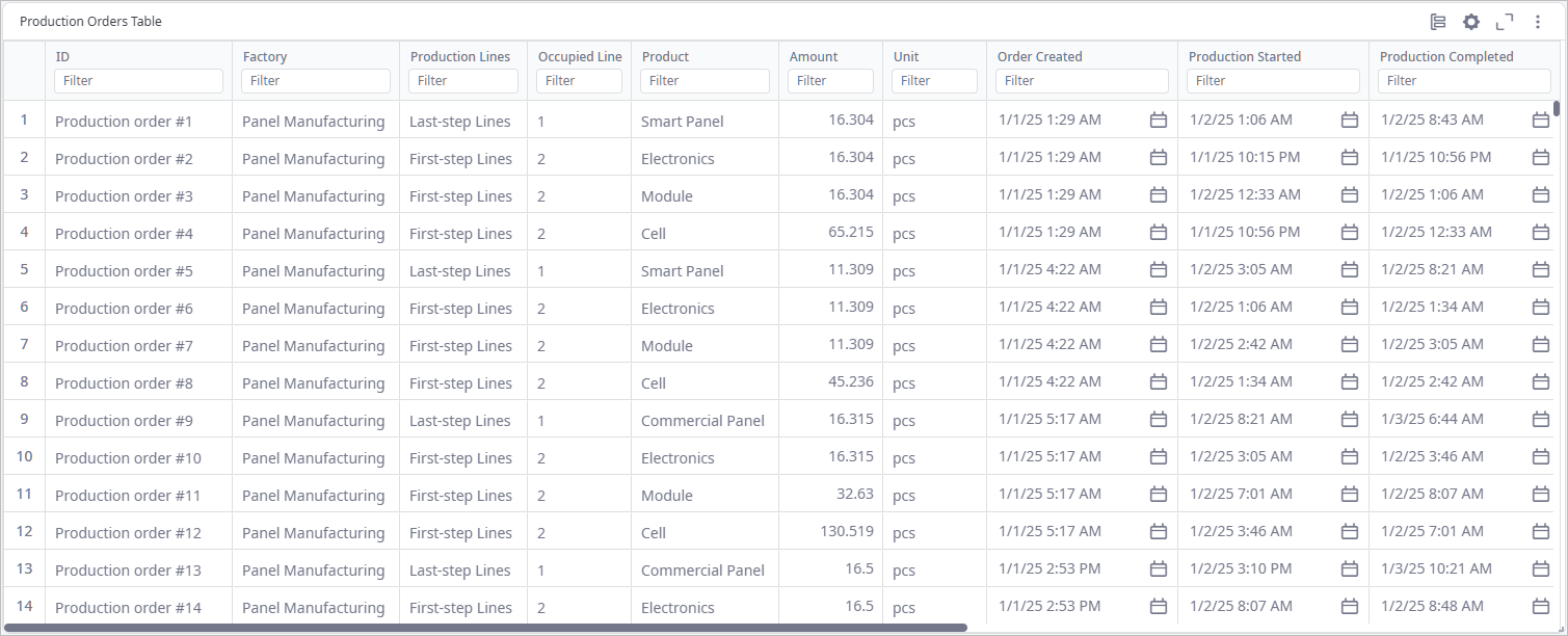
After running the simulation experiment, data on all production orders will be available in the Production Orders Table. Here you can find data on production time, setup times, the number of lines involved in production, etc., of each order.

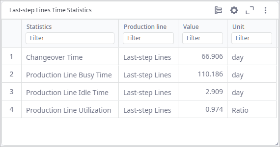
If we look at the Last-Step Lines Time Statistics table chart in the Production Lines dashboard page, we will see that too much time is spent on changeovers.

If we look at the production priorities that are currently defined in the Factories table we will see that:

• The Production Orders Priority is set to FIFO.
• The Product Production Priority is not defined.

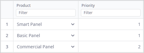
This means that all orders queue for production in the order, in which they arrive at the factory. We will define product priorities by assigning the highest priority to the Commercial Panel product (due to its highest price among the final products).

After this adjustment, we expect production capacity to be focused on the manufacturing of Commercial Panel, allowing other products to share the capacities of the remaining production lines. Since the production order priorities have not been changed, we expect the FIFO order to still apply to the orders within the product-specific queues.

Having run the experiment we can see a reduction in the Changeover Cost KPI metric. This happens because the factory now processes more consecutive orders for the same panel type. As a result, the factory is able to produce more orders, thereby increasing the Revenue metric.

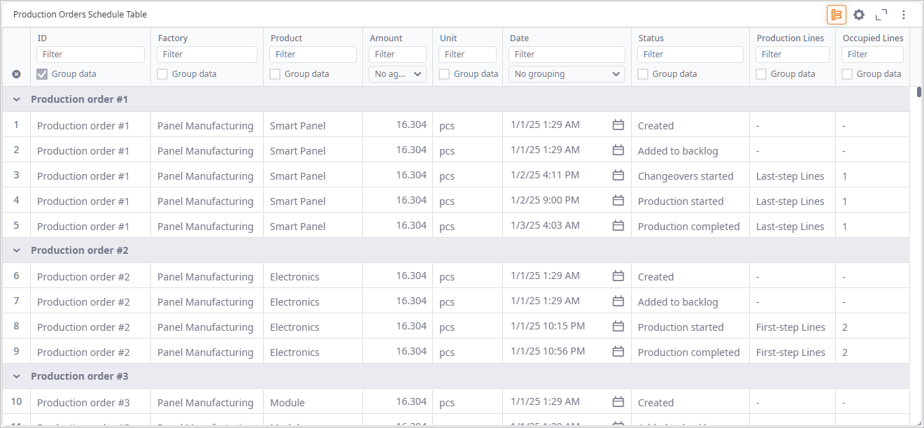
The complete production schedule is available in the Production Orders Schedule statistics. It contains every detail on each status of the order.

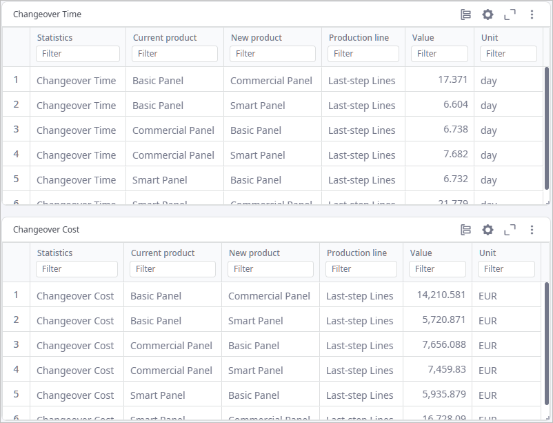
For more details on changeover times and the incurred expenses refer to the Changeover Time and Changeover Cost statistics.

With this scenario we demonstrated the principles of the production system with limited resources and changeover costs. We also obtained a ready-to-use production schedule based on the initial demand data. This simulation example can serve as a foundation for further analysis of management strategies, and production line utilization, as well as assessment of the effect that various production parameters have on the company’s profitability.

How can we improve this article?

Send